Data Science competitions such as Kaggle and KDnuggets have become very popular in recent years. They have real-world data and are a great way to have hands-on practice to gain experience.
When I was in grad school, I took many courses on machine learning and participated in many of these competitions to apply the knowledge that I learned in school. Even after applying so many complicated machine learning and deep-learning algorithms, I was surprised to see the leaderboard when I wasn't even in the 60th percentile.
Why the poor showing? In most of the cases, I was not handling the missing data correctly. That motivated me to learn how to handle missing data the right way.
What is missing data? In simple terms, it's data where values are missing for some of the attributes. Now that we know how important it is to deal with missing data, let's look at five techniques to handle it correctly.
Deductive Imputation
This is an imputation rule defined by logical reasoning, as opposed to a statistical rule. For example, if someone has 2 children in year 1, year 2 has missing values, and 2 children in year 3, we can reasonably impute that they have 2 children in year 2. It requires no inference, and the true value can be assessed. But it can be time-consuming or might require specific coding.
Even though it's accurate, deductive imputation cannot be applied to all datasets. That's why we need to use statistical ways to impute the missing values in some cases.
Let’s apply these methods on an example dataset. We will use the Pima Indians Diabetes dataset (Download from here) which contains medical details including the onset of diabetes within 5 years.
The variable names are as follows: 0. Number of times pregnant.
1. Plasma glucose concentration after 2 hours in an oral glucose tolerance test.
2. Diastolic blood pressure (mm Hg).
3. Triceps skinfold thickness (mm).
4. 2-Hour serum insulin (mu U/ml).
5. Body mass index (weight in kg/(height in m)^2).
6. Diabetes pedigree function.
7. Age (years).
8. Class variable (0 or 1).
These are the first few rows in the dataset.
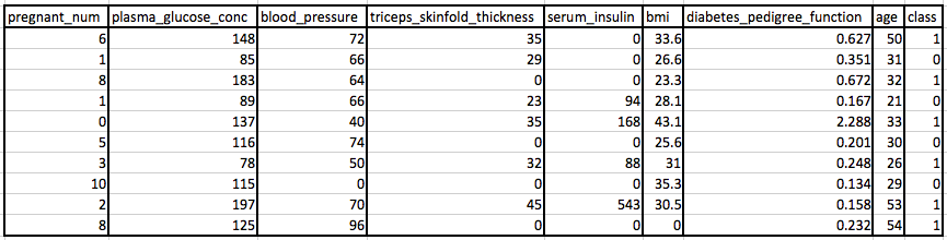
You will notice that there are missing observations for some columns that are marked as a zero value. Specifically, the following columns have an invalid zero value indicating missing values: 1: Plasma glucose concentration
2: Diastolic blood pressure
3: Triceps skinfold thickness
4: 2-Hour serum insulin
5: Body mass index
Mean/Median/Mode Imputation
In this method, any missing values in a given column are replaced with the mean (or median, or mode) of that column. This is the easiest to implement and comprehend. In our example dataset, ‘Triceps skinfold thickness’ is one of the variables that have some missing values. All the missing values in this variable will be replaced by the value 29.12 which is the mean of all the values that are available to us. The same method can be applied to other variables as well.
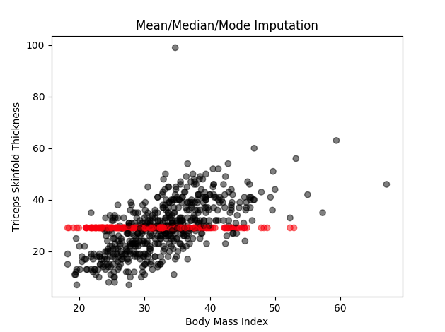
You can see in the diagram, all the missing values have been imputed with the same value.
Regression Imputation
This approach replaces missing values with a predicted value based on a regression line.
Regression is a statistical method which shows the relationship between a dependent variable and independent variables. It's expressed as y = mx + b where m is the slope, b is a constant, x is the independent variable and y is the dependent variable.
In our example, 'Triceps skinfold thickness' is one of the variables where we see some missing values. The missing values in this variable can be imputed by using all other variables information as predictors. It will look like ‘Triceps skinfold thickness’=a + b1(‘Number of times pregnant’) + b2(‘Body Mass Index’) + b3(‘Age’) + ...
In here, we are using all the complete observations of 'Triceps skinfold thickness' variable to predict the missing observations by using 'Number of times pregnant', 'Body Mass Index' and 'Age' as predictors or independent variables. This method assumes that the imputed values fall directly on a regression line with a non-zero slope. As you can see, it is easy to comprehend and seems logical at the same time but it can affect the variability and the distribution of the data to some extent.
A very recommendable R package for regression imputation (and also for other imputation methods) is the mice package. The function mice() is used to impute the data; method = “norm.predict” is the specification for regression imputation, and m = 1 specifies the number of imputed data sets (in our case single imputation).
The code to accomplish that would look something like this:
# regression imputation
imp <- mice(data, method = "norm.predict", m = 1) # Impute data
data_det <- complete(imp) # Store data
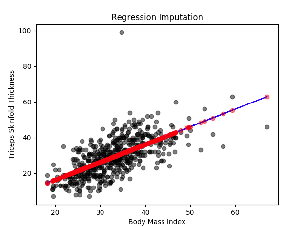
You can see in the diagram all the missing values are imputed based on a regression line using other variables as predictors.
Stochastic Regression Imputation
This aims to preserve the variability of data. To achieve this, we add an error (or residual term) to each predicted score. This residual term is normally distributed with a mean of zero and a variance equal to the variance of the predictor used for imputing.
In the example that we took earlier, it will look like ‘Triceps skinfold thickness’=a + b1(‘Number of times pregnant’) + b2(‘Body Mass Index’) + b3(‘Age’) + ... sigma where sigma is some random error.
We almost use the same code in R for stochastic regression imputation. We only have to change method = “norm.predict” to method = “norm.nob”.
It would look something like this:
# Stochastic regression imputation

imp <- mice(data, method = "norm.nob", m = 1) # Impute data
data_sto <- complete(imp) # Store data
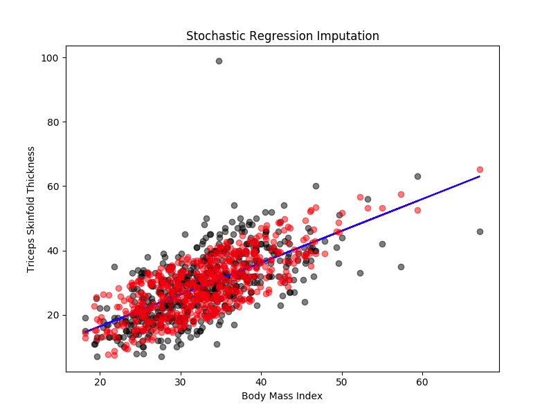
As you can see in the diagram, the missing values are imputed based on the regression line plus some error.
Multiply-Stochastic Regression Imputation
This is similar to singly-stochastic regression imputation (i.e., where the missing values in a given column are replaced with the predicted values based on a regression line and random error), but it is done for a few iterations and the final value is just aggregated by the mean. In our example of imputing missing values in 'Triceps skinfold thickness' variable, we do that the same way we did in stochastic regression imputation (the same R code), but we do it for a few iterations (let's say 10) and we average the predictions to get the final result. It is better than singly-stochastic regression imputation as it allows for much better estimation of true variance. But it takes a bit more effort to implement.
Final Thoughts
As you can see, some methods are quite complex and require a lot of coding. In general, a complex method doesn't necessarily mean it is the best method for all datasets.
In other words, there is no one right method to always use to impute missing values. For example, it is quite possible that deductive imputation could be a much better choice as compared to the regression-based methods in cases where there can be logic applied to impute the missing values.
You can usually guess the right approach in the initial exploratory data analysis phase of your project.